Economics
Interest rates and inflation part 3: Theory
This post takes up from two previous posts (part 1; part 2), asking just what do we (we economists) really know about how interest rates affect inflation….
This post takes up from two previous posts (part 1; part 2), asking just what do we (we economists) really know about how interest rates affect inflation. Today, what does contemporary economic theory say?
As you may recall, the standard story says that the Fed raises interest rates; inflation (and expected inflation) don’t immediately jump up, so real interest rates rise; with some lag, higher real interest rates push down employment and output (IS); with some more lag, the softer economy leads to lower prices and wages (Phillips curve). So higher interest rates lower future inflation, albeit with “long and variable lags.”
Higher interest rates -> (lag) lower output, employment -> (lag) lower inflation.
In part 1, we saw that it’s not easy to see that story in the data. In part 2, we saw that half a century of formal empirical work also leaves that conclusion on very shaky ground.
As they say at the University of Chicago, “Well, so much for the real world, how does it work in theory?” That is an important question. We never really believe things we don’t have a theory for, and for good reason. So, today, let’s look at what modern theory has to say about this question. And they are not unrelated questions. Theory has been trying to replicate this story for decades.
The answer: Modern (anything post 1972) theory really does not support this idea. The standard new-Keynesian model does not produce anything like the standard story. Models that modify that simple model to achieve something like result of the standard story do so with a long list of complex ingredients. The new ingredients are not just sufficient, they are (apparently) necessary to produce the desired dynamic pattern. Even these models do not implement the verbal logic above. If the pattern that high interest rates lower inflation over a few years is true, it is by a completely different mechanism than the story tells.
I conclude that we don’t have a simple economic model that produces the standard belief. (“Simple” and “economic” are important qualifiers.)
The simple new-Keynesian model
The central problem comes from the Phillips curve. The modern Phillips curve asserts that price-setters are forward-looking. If they know inflation will be high next year, they raise prices now. So
Inflation today = expected inflation next year + (coefficient) x output gap.
[pi_t = E_tpi_{t+1} + kappa x_t](If you know enough to complain about (betaapprox0.99) in front of (E_tpi_{t+1}) you know enough that it doesn’t matter for the issues here.)
Now, if the Fed raises interest rates, and if (if) that lowers output or raises unemployment, inflation today goes down.
The trouble is, that’s not what we’re looking for. Inflation goes down today, ((pi_t))relative to expected inflation next year ((E_tpi_{t+1})). So a higher interest rate and lower output correlate with inflation that is rising over time.
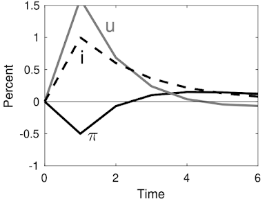
Here is a concrete example:

The plot is the response of the standard three equation new-Keynesian model to an (varepsilon_1) shock at time 1:[begin{align} x_t &= E_t x_{t+1} – sigma(i_t – E_tpi_{t+1}) \ pi_t & = beta E_t pi_{t+1} + kappa x_t \ i_t &= phi pi_t + u_t \ u_t &= eta u_{t-1} + varepsilon_t. end{align}] Here (x) is output, (i) is the interest rate, (pi) is inflation, (eta=0.6), (sigma=1), (kappa=0.25), (beta=0.95), (phi=1.2).
In this plot, higher interest rates are said to lower inflation. But they lower inflation immediately, on the day of the interest rate shock. Then, as explained above, inflation rises over time.
In the standard view, and the empirical estimates from the last post, a higher interest rate has no immediate effect, and then future inflation is lower. See plots in the last post, or this one from Romer and Romer’s 2023 summary:

Inflation jumping down and then rising in the future is quite different from inflation that does nothing immediately, might even rise for a few months, and then starts gently going down.
You might even wonder about the downward jump in inflation. The Phillips curve makes it clear why current inflation is lower than expected future inflation, but why doesn’t current inflation stay the same, or even rise, and expected future inflation rise more? That’s the “equilibrium selection” issue. All those paths are possible, and you need extra rules to pick a particular one. Fiscal theory points out that the downward jump needs a fiscal tightening, so represents a joint monetary-fiscal policy. But we don’t argue about that today. Take the standard new Keynesian model exactly as is, with passive fiscal policy and standard equilibrium selection rules. It predicts that inflation jumps down immediately and then rises over time. It does not predict that inflation slowly declines over time.
This is not a new issue. Larry Ball (1994) first pointed out that the standard new Keynesian Phillips curve says that inflation is high when inflation is high relative to expected future inflation, that is when inflation is declining. Standard beliefs go the other way: output is high when inflation is rising.
The IS curve is a key part of the overall prediction, and output faces a similar problem. I just assumed above that output falls when interest rates rise. In the model it does; output follows a path with the same shape as inflation in my little plot. Output also jumps down and then rises over time. Here too, the (much stronger) empirical evidence says that an interest rate rise does not change output immediately, and output then falls rather than rises over time. The intuition has even clearer economics behind it: Higher real interest rates induce people to consume less today and more tomorrow. Higher real interest rates should go with higher, not lower, future consumption growth. Again, the model only apparently reverses the sign by having output jump down before rising.
Key issues
How can we be here, 40 years later, and the benchmark textbook model so utterly does not replicate standard beliefs about monetary policy?
One answer, I believe, is confusing adjustment to equilibrium with equilibrium dynamics. The model generates inflation lower than yesterday (time 0 to time 1) and lower than it otherwise would be (time 1 without shock vs time 1 with shock). Now, all economic models are a bit stylized. It’s easy to say that when we add various frictions, “lower than yesterday” or “lower than it would have been” is a good parable for “goes down over time.” If in a simple supply and demand graph we say that an increase in demand raises prices instantly, we naturally understand that as a parable for a drawn out period of price increases once we add appropriate frictions.
But dynamic macroeconomics doesn’t work that way. We have already added what was supposed to be the central friction, sticky prices. Dynamic economics is supposed to describe the time-path of variables already, with no extra parables. If adjustment to equilibrium takes time, then model that.
The IS and Phillips curve are forward looking, like stock prices. It would make little sense to say “news comes out that the company will never make money, so the stock price should decline gradually over a few years.” It should jump down now. Inflation and output behave that way in the standard model.
A second confusion, I think, is between sticky prices and sticky inflation. The new-Keynesian model posits, and a huge empirical literature examines, sticky prices. But that is not the same thing as sticky inflation. Prices can be arbitrarily sticky and inflation, the first derivative of prices, can still jump. In the Calvo model, imagine that only a tiny fraction of firms can change prices at each instant. But when they do, they will change prices a lot, and the overall price level will start increasing right away. In the continuous-time version of the model, prices are continuous (sticky), but inflation jumps at the moment of the shock.
The standard story wants sticky inflation. Many authors explain the new-Keynesian model with sentences like “the Fed raises interest rates. Prices are sticky, so inflation can’t go up right away and real interest rates are higher.” This is wrong. Inflation can rise right away. In the standard new-Keynesian model it does so with (eta=1), for any amount of price stickiness. Inflation rises immediately with a persistent monetary policy shock.
Just get it out of your heads. The standard model does not produce the standard story.
The obvious response is, let’s add ingredients to the standard model and see if we can modify the response function to look something like the common beliefs and VAR estimates. Let’s go.
Adaptive expectations
We can reproduce standard beliefs about monetary policy with thoroughly adaptive expectations, in the 1970s ISLM form. I think this is a large part of what most policy makers and commenters have in mind.
Modify the above model to leave out the dynamic part of the intertemporal substitution equation, to just say in rather ad hoc way that higher real interest rates lower output, and specify that the expected inflation that drives the real rate and that drives pricing decisions is mechanically equal to previous inflation, (E_t pi_{t+1} = pi_{t-1}). We get [ begin{align} x_t &= -sigma (i_t – pi_{t-1}) \ pi_t & = pi_{t-1} + kappa x_t .end{align}] We can solve this sytsem analytically to [pi_t = (1+sigmakappa)pi_{t-1} + sigmakappa i_t.]

Here’s what happens if the Fed permanently raises the interest rate. Higher interest rates send future inflation down. ((kappa=0.25, sigma=1.)) Inflation eventually spirals away, but central banks don’t leave interest rates alone forever. If we add a Taylor rule response (i_t = phi pi_t + u_t), so the central bank reacts to the emerging spiral, we get this response to a permanent monetary policy disturbance (u_t):

The higher interest rate sets off a deflation spiral. But the Fed quickly follows inflation down to stabilize the situation. This is, I think, the conventional story of the 1980s.

- Habit formation. The utility function is (log(c_t – bc_{t-1})).
- A capital stock with adjustment costs in investment. Adjustment costs are proportional to investment growth, ([1-S(i_t/i_{t-1})]i_t), rather than the usual formulation in which adjustment costs are proportional to the investment to capital ratio (S(i_t/k_t)i_t).
- Variable capital utilization. Capital services (k_t) are related to the capital stock (bar{k}t) by (k_t = u_t bar{k}_t). The utilization rate (u_t) is set by households facing an upward sloping cost (a(u_t)bar{k}_t).
- Calvo pricing with indexation: Firms randomly get to reset prices, but firms that aren’t allowed to reset prices do automatically raise prices at the rate of inflation.
- Prices are also fixed for a quarter. Technically, firms must post prices before they see the period’s shocks.
- Sticky wages, also with indexation. Households are monopoly suppliers of labor, and set wages Calvo-style like firms. (Later papers put all households into a union which does the wage setting.) Wages are also indexed; Households that don’t get to reoptimize their wage still raise wages following inflation.
- Firms must borrow working capital to finance their wage bill a quarter in advance, and thus pay a interest on the wage bill.
- Money in the utility function, and money supply control. Monetary policy is a change in the money growth rate, not a pure interest rate target.
… the interest rate appears in firms’ marginal cost. Since the interest rate drops after an expansionary monetary policy shock, the model embeds a force that pushes marginal costs down for a period of time. Indeed, in the estimated benchmark model the effect is strong enough to induce a transient fall in inflation.
This is about where we are. Despite the pretty response functions, I still score that we don’t have a reliable, simple, economic model that produces the standard view of monetary policy.
Mankiw and Reis, sticky expectations
Mankiw and Reis (2002) expressed the challenge clearly over 20 years ago. In reference to the “standard” New-Keynesian Phillips curve (pi_t = beta E_t pi_{t+1} + kappa x_t) they write a beautiful and succinct paragraph:
Ball [1994a] shows that the model yields the surprising result that announced, credible disinflations cause booms rather than recessions. Fuhrer and Moore [1995] argue that it cannot explain why inflation is so persistent. Mankiw [2001] notes that it has trouble explaining why shocks to monetary policy have a delayed and gradual effect on inflation. These problems appear to arise from the same source: although the price level is sticky in this model, the inflation rate can change quickly. By contrast, empirical analyses of the inflation process (e.g., Gordon [1997]) typically give a large role to “inflation inertia.”
At the cost of repetition, I emphasize the last sentence because it is so overlooked. Sticky prices are not sticky inflation. Ball already said this in 1994:
Taylor (1979, 198) and Blanchard (1983, 1986) show that staggering produces inertia in the price level: prices just slowly to a fall in th money supply. …Disinflation, however, is a change in the growth rate of money not a one-time shock to the level. In informal discussions, analysts often assume that the inertia result carries over from levels to growth rates — that inflation adjusts slowly to a fall in money growth.
As I see it, Mankiw and Reis generalize the Lucas (1972) Phillips curve. For Lucas, roughly, output is related to unexpected inflation[pi_t = E_{t-1}pi_t + kappa x_t.] Firms don’t see everyone else’s prices in the period. Thus, when a firm sees an unexpected rise in prices, it doesn’t know if it is a higher relative price or a higher general price level; the firm expands output based on how much it thinks the event might be a relative price increase. I love this model for many reasons, but one, which seems to have fallen by the wayside, is that it explicitly founds the Phillips curve in firms’ confusion about relative prices vs. the price level, and thus faces up to the problem why should a rise in the price level have any real effects.
Mankiw and Reis basically suppose that firms find out the general price level with lags, so output depends on inflation relative to a distributed lag of its expectations. It’s clearest for the price level (p. 1300)[p_t = lambdasum_{j=0}^infty (1-lambda)^j E_{t-j}(p_t + alpha x_t).] The inflation expression is [pi_t = frac{alpha lambda}{1-lambda}x_t + lambda sum_{j=0}^infty (1-lambda)^j E_{t-1-j}(pi_t + alpha Delta x_t).](Some of the complication is that you want it to be (pi_t = sum_{j=0}^infty E_{t-1-j}pi_t + kappa x_t), but output doesn’t enter that way.)
This seems totally natural and sensible to me. What is a “period” anyway? It makes sense that firms learn heterogeneously whether a price increase is relative or price level. And it obviously solves the central persistence problem with the Lucas (1972) model, that it only produces a one-period output movement. Well, what’s a period anyway? (Mankiw and Reis don’t sell it this way, and actually don’t cite Lucas at all. Curious.)
It’s not immediately obvious that this curve solves the Ball puzzle and the declining inflation puzzle, and indeed one must put it in a full model to do so. Mankiw and Reis (2002) mix it with (m_t + v = p_t + x_t) and make some stylized analysis, but don’t show how to put the idea in models such as I started with or make a plot.
Their less well known follow on paper Sticky Information in General Equilibrium (2007) is much better for this purpose because they do show you how to put the idea in an explicit new-Keynesian model, like the one I started with. They also add a Taylor rule, and an interest rate rather than money supply instrument, along with wage stickiness and a few other ingredients,. They show how to solve the model overcoming the problem that there are many lagged expectations as state variables. But here is the response to the monetary policy shock:
 |
| Response to a Monetary Policy Shock, Mankiw and Reis (2007). |
Sadly they don’t report how interest rates respond to the shock. I presume interest rates went down temporarily.
Look: the inflation and output gap plots are about the same. Except for the slight delay going up, these are exactly the responses of the standard NK model. When output is high, inflation is high and declining. The whole point was to produce a model in which high output level would correspond to rising inflation. Relative to the first graph, the main improvement is just a slight hump shape in both inflation and output responses.
Describing the same model in “Pervasive Stickiness” (2006), Mankiw and Reis describe the desideratum well:
The Acceleration Phenomenon….inflation tends to rise when the economy is booming and falls when economic activity is depressed. This is the central insight of the empirical literature on the Phillips curve. One simple way to illustrate this fact is to correlate the change in inflation, (pi_{t+2}-pi_{t-2}) with [the level of] output, (y_t), detrended with the HP filter. In U.S. quarterly data from 1954-Q3 to 2005-Q3, the correlation is 0.47. That is, the change in inflation is procyclical.
Now look again at the graph. As far as I can see, it’s not there. Is this version of sticky inflation a bust, for this purpose?
I still think it’s a neat idea worth more exploration. But I thought so 20 years ago too. Mankiw and Reis have a lot of citations but nobody followed them. Why not? I suspect it’s part of a general pattern that lots of great micro sticky price papers are not used because they don’t produce an easy aggregate Phillips curve. If you want cites, make sure people can plug it in to Dynare. Mankiw and Reis’ curve is pretty simple, but you still have to keep all past expectations around as a state variable. There may be alternative ways of doing that with modern computational technology, putting it in a Markov environment or cutting off the lags, everyone learns the price level after 5 years. Hank models have even bigger state spaces!
Some more models
What about within the Fed? Chung, Kiley, and Laforte 2010, “Documentation of the Estimated, Dynamic, Optimization-based (EDO) Model of the U.S. Economy: 2010 Version” is one such model. (Thanks to Ben Moll, in a lecture slide titled “Effects of interest rate hike in U.S. Fed’s own New Keynesian model”) They describe it as
This paper provides documentation for a large-scale estimated DSGE model of the U.S. economy – the Federal Reserve Board’s Estimated, Dynamic, Optimization- based (FRB/EDO) model project. The model can be used to address a wide range of practical policy questions on a routine basis.
Here are the central plots for our purpose: The response of interest rates and inflation to a monetary policy shock.

No long and variable lags here. Just as in the simple model, inflation jumps down on the day of the shock and then reverts. As with Mankiw and Reis, there is a tiny hump shape, but that’s it. This is nothing like the Romer and Romer plot.

I’ll reiterate the main point. As far as I can tell, there is no simple economic model that produces the standard belief.
Now, maybe belief is right and models just have to catch up. It is interesting that there is so little effort going on to do this. As above, the vast outpouring of new-Keynesian modeling has been to add even more ingredients. In part, again, that’s the natural pressures of journal publication. But I think it’s also an honest feeling that after Christiano Eichenbaun and Evans, this is a solved problem and adding other ingredients is all there is to do.
So part of the point of this post (and “Expectations and the neutrality of interest rates“) is to argue that this is not a solved problem, and that removing ingredients to find the simplest economic model that can produce standard beliefs is a really important task. Then, does the model incorporate anything at all of the standard intuition, or is it based on some different mechanism al together? These are first order important and unresolved questions!
But for my lay readers, here is as far as I know where we are. If you, like the Fed, hold to standard beliefs that higher interest rates lower future output and inflation with long and variable lags, know there is no simple economic theory behind that belief, and certainly the standard story is not how economic models of the last four decades work.
inflation
deflation
monetary
reserve
policy
money supply
interest rates
fed
central bank
correlation
expansionary
monetary policy


Argentina Is One of the Most Regulated Countries in the World
In the coming days and weeks, we can expect further, far‐reaching reform proposals that will go through the Argentine congress.

Crypto, Crude, & Crap Stocks Rally As Yield Curve Steepens, Rate-Cut Hopes Soar
Crypto, Crude, & Crap Stocks Rally As Yield Curve Steepens, Rate-Cut Hopes Soar
A weird week of macro data – strong jobless claims but…
Fed Pivot: A Blend of Confidence and Folly
Fed Pivot: Charting a New Course in Economic Strategy Dec 22, 2023 Introduction In the dynamic world of economics, the Federal Reserve, the central bank…